Overview
This section collects end-to-end tutorials for each combination of sampler and estimator available in GLIDE. Each tutorial walks through a complete path from sampling to annotation to estimation on a simulated dataset, so you can follow along with the use case that best matches your own.
If you are new to GLIDE, read the User Guide first: it explains the three-stage pipeline and the role of each component. The guidance below helps you pick the right sampler and estimator for each stage of that workflow.
Choosing the right sampler and estimator
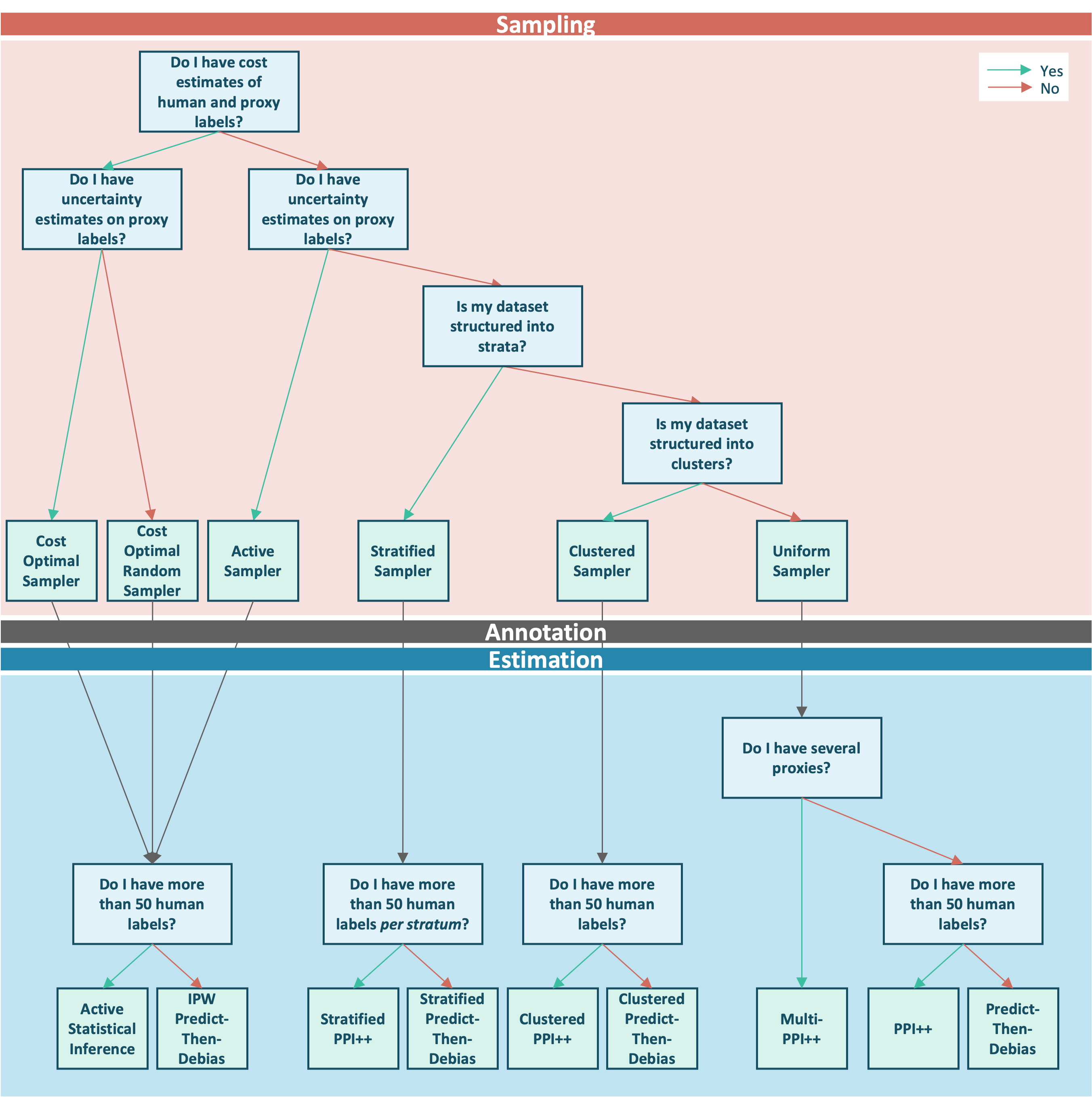
The workflow breaks into three sequential phases: Sampling (deciding which items to send for human annotation), Annotation (collecting human labels), and Estimation (computing debiased statistics from the combined human and proxy data). The decision tree below guides you through each phase.
Phase 1: Sampling
Before any human annotation takes place, you must decide how to select the items that will be sent for review. Four questions determine the right sampler.
1. Do you have cost estimates of human and proxy labels? If you know (or can estimate) the cost per human annotation and the cost of obtaining a proxy label, GLIDE can allocate your annotation budget optimally rather than uniformly. This unlocks the cost-aware samplers, which minimise the variance of downstream estimates for a fixed budget.
2. Do you have uncertainty estimates on proxy labels? If your proxy model outputs a confidence score or probability alongside each label, the sampling probabilities can be derived from these scores. Uncertainty-aware sampling concentrates human review on the items where the proxy is least reliable, improving statistical efficiency.
3. Is your dataset structured into strata? If your data partitions naturally into groups (by language, domain, question type, etc.) and you expect the proxy model to behave differently across groups, a stratified sampling strategy ensures that each group is represented in the annotated set.
4. Is your dataset structured into clusters? If your samples are grouped into clusters of correlated items (sentences within a paragraph, turns within a conversation, etc.) that must be annotated together as a unit, a clustered sampling strategy draws whole clusters rather than individual samples and defines the annotation budget in terms of clusters. This keeps the statistical inference valid in the presence of within-cluster correlation.
Phase 2: Annotation
Once a sample has been selected, human annotators label the chosen items. The size of this annotated set relative to your strata is the key quantity for the estimation phase.
Phase 3: Estimation
With human labels in hand, two questions determine the estimator.
Do you have several proxy sources? If more than one proxy annotator (for example, two different LLM judges) labelled every item, Multi-PPI++ combines all of them into a single debiased estimate, learning the optimal weight for each source from the labeled data. A source that agrees more closely with the human annotations receives a larger weight, and the result is always at least as efficient as using human labels alone.
Do you have more than 50 human labels (per stratum for stratified methods)? PPI and Active Statistical Inference form the CLT-family, they rely on normal approximations to construct confidence intervals. This approximation requires a sufficient number of labeled samples, typically at least 50 per stratum (or in total for non-stratified methods). Below this threshold, the Predict-Then-Debias bootstrap family of estimators provides a simpler and more conservative alternative that remains valid with fewer annotations.
Available tutorials
Each tutorial walks through one complete path in the above decision tree: from sampling to annotation to estimation, on a simulated dataset. Use the table below to find the tutorial that matches your situation.
| Cost estimates? | Uncertainty scores? | Stratified data? | Clustered data? | Multiple proxies? | Phase 1 sampler | Phase 3 estimator | Tutorial |
|---|---|---|---|---|---|---|---|
| No | No | No | No | No | Uniform random | PPI++ | Standard annotation budget (PPI++) |
| No | No | No | No | Yes | Uniform random | Multi-PPI++ | Multiple proxies (Multi-PPI++) |
| No | No | Yes | No | No | Stratified uniform | Stratified PPI++ | Stratified data (Stratified PPI++) |
| No | No | No | Yes | No | Clustered uniform | Clustered PPI++ | Clustered data (Clustered PPI++) |
| No | Yes | No | No | No | Uncertainty-aware | ASI | Uncertainty scores available (ASI) |
| Yes | No | No | No | No | Cost-optimal random | PPI++ | Cost estimates available (Cost-Optimal Random Sampling) |
| Yes | Yes | No | No | No | Cost-optimal | ASI | Cost and uncertainty scores available (Cost-Optimal Sampling) |
If your data contains fewer than 50 human labels: use the PTD variant of the estimators above (PTDMeanEstimator for PPI++, StratifiedPTDMeanEstimator for Stratified PPI++, ClusteredPTDMeanEstimator for Clustered PPI++, and IPWPTDMeanEstimator for ASI). In the stratified case, the StratifiedPTDMeanEstimator should be used whenever one of the strata has fewer than 50 labels. The tutorial workflow for the respective estimators is identical; only the estimator class changes.
Monitoring a deployed system for drift
Once a system is deployed, the question shifts from estimating a metric once to watching it over time: has it drifted past an acceptable threshold? This is a different problem from the sampler/estimator selection above, since it is not about a one-off estimate but about re-estimating a metric on successive batches of production data while keeping repeated checks statistically valid. The Monitoring a deployed system for drift (PPRM) tutorial walks through this post-deployment workflow with EmpiricalPPIMeanMonitor.