Evaluation Workflow

This page explains how to plan and execute a rigorous evaluation with GLIDE, from raw data to a valid, unbiased metric estimate.

The evaluation problem

Suppose you have an AI system that produces answers over a large dataset of \(N\) samples, and you want to measure its performance, for example its accuracy, relevance score, or any other scalar metric \(\theta^*\).

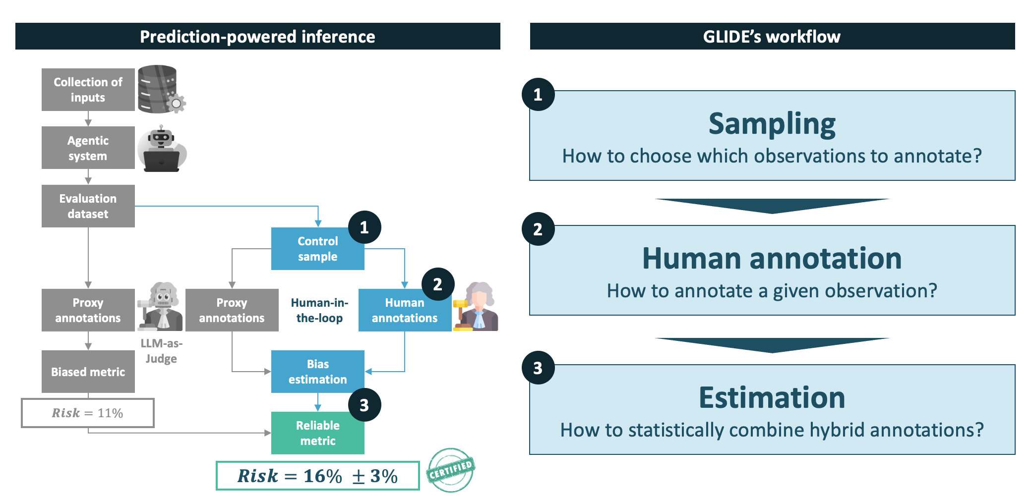
Computing \(\theta^*\) exactly requires reliable annotations \(Y\) for every sample. Human annotations are reliable but expensive, so in practice you only label a small subset of \(n \ll N\) samples. A natural shortcut is to use proxy labels \(\tilde{Y}\) (automated predictions from, for example, an LLM-as-Judge) to cover all \(N\) samples cheaply. The problem: proxy labels are generally biased (\(E[\tilde{Y}] \neq \theta^*\)), so naively averaging them gives a systematically wrong estimate of \(\theta^*\).

GLIDE addresses this by combining large pools of cheap proxy labels with small sets of human labels to produce unbiased, reliable estimates of \(\theta^*\). By combining these two sources, GLIDE can achieve the same statistical precision as a purely human-labeled approach, at a fraction of the annotation cost. Actual savings depend on the annotation effort required and how well the proxy aligns with human judgement, but the potential gains can be substantial. This makes rigorous performance evaluation tractable even for large-scale AI systems.

The workflow has three stages:

GLIDE's workflow

Do you need a sampler?

If you already have human labels for a uniformly drawn random subset of the data (for example, from a pre-existing annotation campaign), you can skip the sampling stage entirely and go straight to the estimator.

A sampler is useful when you still need to allocate an annotation budget and want to do so in the most efficient way to reduce downstream estimation uncertainty. A naive uniform sampling strategy may lead to sub-optimal annotation budget allocation in this regard.

Stage 1: Sampling

You start with a fully proxy-labeled dataset. The sampler's job is to assign a sampling probability \(\pi_i\) to each sample and to select \(b\) samples for human annotation where \(b\) represents an annotation budget to be allocated. The probabilities \(\pi_i\) are needed by the downstream estimator to correct for non-uniform selection.

Guided sampling

Samplers can exploit the structure of the data or auxiliary information to allocate the annotation budget more efficiently. For example, a sampler may use predefined strata to ensure balanced coverage across subgroups, or it may rely on per-instance auxiliary signals (such as proxy label uncertainty) to focus annotation on the most informative samples.

Choosing a sampler

GLIDE provides multiple samplers. The choice depends on the structure of your data, for example, whether it can be split into naturally defined groups (language, domain, topic, ...) or whether per-sample uncertainty scores are available. See Samplers for a full description of each option.

Samplers compute drawing probabilities for each sample. These are used to select samples for human annotation by setting an indicator value for each element. The probabilities and indicator values are directly used by downstream estimators.

Stage 2: Human annotation

The selected samples (\(\xi_i = 1\)) must be labeled by humans before estimation can proceed. This is typically handled through an annotation process, where annotators are presented with each item and record their judgements according to a predefined rubric.

For many evaluation tasks, such as assessing factual accuracy, safety, or subtle reasoning, the annotation requires genuine expertise: annotators must be qualified to make reliable judgements on the items at hand. Expert annotation is accurate, but calling upon it comes at a cost, which is why allocating the annotation budget efficiently matters.

Once all selected samples have been labeled, you have everything needed to run the estimator.

Stage 3: Estimation

Once human labels \(Y_i\) have been collected for samples with \(\xi_i = 1\), the estimator combines them with the proxy labels to produce an unbiased mean estimate and a confidence interval.

Choosing an estimator

The right estimator depends on how the labeled subset was drawn:

How were labels collected?	Recommended estimator
Uniform random sample (no sampler used)	PPI++
Stratified sampling via `StratifiedSampler` with proportional allocation	Stratified PPI++
Non-uniform sampling via `ActiveSampler` or `StratifiedSampler` with Neyman allocation	ASI
No proxy labels available; human labels only	Classical

See Estimators for a full description of each option.

Full workflow example

Here is a concrete end-to-end sequence for a scenario where the data has natural strata (e.g., languages) and you want to allocate an annotation budget of \(b = 200\):

Proxy-label all \(N\) samples with your automated judge.
Run StratifiedSampler with Neyman allocation and \(b = 200\). This sets \(\pi_i\) and \(\xi_i\) for every sample with \(\xi_i = 1\) for 200 samples at most.
Collect human annotations \(Y_i\) for each sample where \(\xi_i = 1\) through your annotation process.
Run StratifiedPPI on the full dataset where each sample has a proxy \(\tilde{Y}_i\), and the ground truths \(Y_i\) are present for labeled samples.
Read the point estimate \(\hat{\theta}\) and the confidence interval \([\hat{\theta} - \delta, \hat{\theta} + \delta]\) for a desired confidence level.

If instead labels already exist for a uniform random subset, skip steps 2–3 and run Stratified PPI++ directly.

See also the Stratified PPI tutorial for a worked example.